Introduction
In this "Instructable" I will show you how to measure vibrations around you. You might ask: why do I need that?
Well, there are endless applications towards that, but several handy examples would be: knowing if someone is at home or not, is the motor going to breakdown soon, or if there are earthquakes and what's their magnitude, to name a few. Raising the vibrations awareness can help to design smart anti-theft systems, or predict malfunctioning before it happens and a lot more. Also it can help you to learn more practical stuff and use it, rather a pure theory as in school or university.
We will measure vibrations that are travelling from excitation source which is a running brushed DC-motor. That will give you a background to explore further and expand on other sources.
To accomplish our goal, there are several methods. One would be: to get a 3-axis accelerometer IC, and develop a PCB which then will measure the g-forces across this axes, and notify to micro-controller via SPI, or I2C. There are very sensitive ICs which are capable of measuring with up to 24-Bit resolution and require a lot of infrastructure and development to function properly, normally these would be suitable more for industrial or scientific usage. The scope of this Intractable is to work with more affordable and easy to use technology and learn something along the way. Therefore we will skip the above method and use “KenjiX1” robot and a conductive vibration scanning probe from “Physalis Labs”. Mostly all the types of sensors and probes and in general most of the IC's as well as sensors are made on basis of piezoelectric effect discovered by Pierre and Marie Curie.
The probes that utilizes KenjiX1 are easy to use, and even if they brake, you can replace it with minor effort. There are several types of probes available, and the difference is basically the probe geometry, which is then applied to the surface and is designed in a way that it creates a good contact with the surface and that way the waves are travelling with less effort through one body (surface) to the another (probe).
KenjiX1 robot can utilize several types of vibration measuring types of probes. For our tests, we will employ the flat probe (Fig.1). It’s meant to be used for surfaces which are flat or glassy, walls and everything that will fall into that category, basically on everything that is flat.

Fig.1. Conductive probe with a rounded flat disc on it meant for flat surfaces.
Supplies and Consumables….
Instruments, Tools, and Supplies:
----------------------------------
- Laptop with terminal programs (Putty and TeraTerm) (any Linux, MacOS or Windows Machine).
- KenjiX1 open-source tele-robotics platform http://physalislabs.org/projects/kenjix1/ Vibration measurement Probe (flat surface geometry) from http://physalislabs.org/
- OriginLab Software for data evaluation. https://www.originlab.com/
- Adjustable laboratory power supply or just batteries to power the motor.
- Brushed DC-motor.
Let's start with a short description of each step:
- Install a terminal software https://ttssh2.osdn.jp/index.html.en (TerraTerm, Putty, for windows, and Xterm or similar for Linux). Here I will be using TeraTerm because I am working on Windows machine at the moment. But you can just pick your favorite terminal software for your suitable machine.
- Kenji X1 platform conductive-probe (flat surface) courtesy of "Physalis Labs". You can purchase them or submit your request for trying them out through the website: http://physalislabs.org/projects/kenjix1/,or just back their crowdfunding campaign on Kickstarter, that way you will receive the Kenji X1 and complete kit with supercheap price, also helping out the folks at Physalis labs to spread their word around the world.
- Go to OriginLab website and download the installer, and then install the “OriginLab” software from https://www.originlab.com/. Normally it’s paid, but you can use the trial for a month. Later you can decide to keep it, to or remove it. This software is more related to Windows machines, but they have a guide how to run it on Macs here: https://www.originlab.com/index.aspx?go=Support/DocumentationAndHelpCenter/Installation/RunOriginonaMac
- Regular laboratory power supply which will be capable of powering any of the above mentioned motors will be fine, or just use batteries, please make sure you use the correct voltage for the motor.
- Brushed DC-Motor scavenged from broken electronics or other similar devices would be an option too. Make sure that the voltage of the motor and the power-supply/batteries is in working range of the motor, otherwise it will not run, or if does, will be very slow, in case of voltage being below the spec, or will run superfast and might break if being too high above the spec. That’s if for the materials and tools….Now we can finally nosedive into our study of acquiring vibration profile of running Brushed DC-motor.
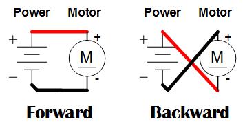
Fig.2. Wiring the brushed DC-motor with the suitable power source.
Vibrations Nosedive
Vibrations are everywhere, they occur around us and in nature heavily. Therefore it is crucial to understand their source and reasons for them to occur. An ongoing monitoring of vibrations keeps awareness on possible earthquakes and other natural disasters occurrences.
On the other hand, monitoring of various vibrations and their magnitude aka amplitude can help prevent failures and down-times of machinery and complex systems which are constantly online and working around us. In power-plants, factories, production lines ongoing verification of the vibrations noise floor is needed. For all hardware, mechatronic and mechanic systems which are running, to keep the awareness on their wear and tear. Not only can it help save maintenance costs, but also painful down-times which can occur due to unexpected breakdown of such complex hardware systems and causing further issues, down the line.
Normally this topic has a huge support in physics, and other natural science disciplines, and heavy math (°_°). Here, I we will skip that and get more physical on real world applications.
Normally vibrations are measured in two domains, time and frequency.
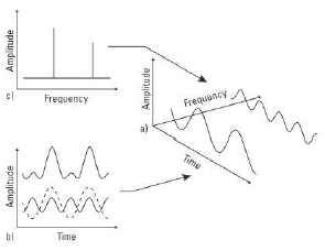
Fig.3. Graphical representation of several excitation sources c (amplitude vs. frequency), b (amplitude vs. time), a (amplitude vs. frequency and time).
As represented in (Fig.3.) the excitation source can generate waves which can look as sinusoids, with high or low frequencies or sharp peaks which occur instantaneously. We can measure the waves incoming in two domains: time, which means the effect/wave is being observed as time changes Fig.3. (b), and the frequency, which means that we observe the effect/wave’s power as the frequency changes Fig.3.(c). You would need to apply a Fourier transform to move from Fig.3.(b) to Fig.3.(c).
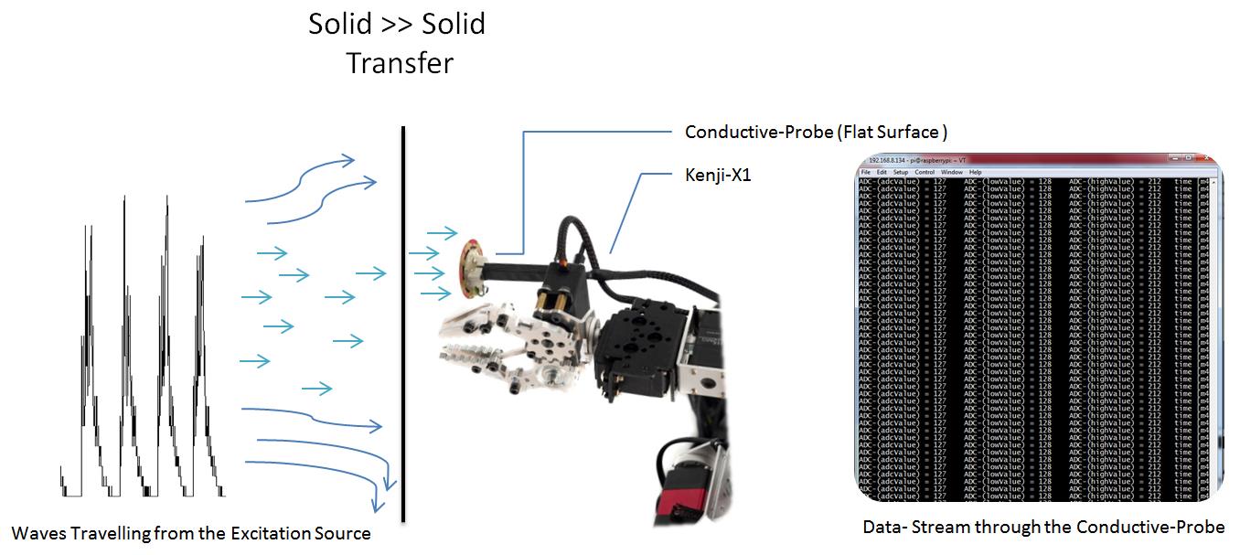
Fig.4. Illustration of the vibration waves travelling through a conductive-probe from excitation source into KenjiX1.
I have created an illustration of how the waves caused by some excitation (human typing on keyboard, hammer, DC-motor etc…) are travelling through a matter (solid, liquid, gas) getting from one solid object (wall, table, metal and stairs) to another solid object, which happens to be our conductive-probe. The super flat and wide surface of the probe creates a proper contact with the other flat surface, which enables the waves to cross through with less effort, which at the same time is a prerequisite for a good signal acquisition.
Further the conductive-probe directs the signal to the KenjiX1 platform where it gets registered by the onboard CPU, or shuttled further for processing.
For measuring the vibrations remotely, I am using the KenjiX1 robot platform from Physalis Labs. It is really an awesome robotics development open-source platform which overlaps the gap between the industrial robotics farcry and the maker/tinkerer level smallish ones. More information on KenjiX1 can be found here http://physalislabs.org/projects/kenji/.
Starting Up Kenji X1…
So far we’ve got through the introduction and the uses of vibrational waves, then we went briefly over the tools and materials to complete the task, and lastly some theory and information which will help us understand what exactly is happening behind the curtains. Now we start with the actual experimental stuff ahead. Start your laptop/PC and connect to the WLAN which is available to you and to Kenji X1.
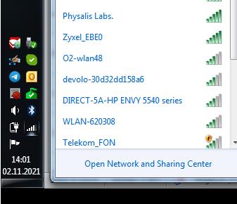
Fig.5. Connecting to a WLAN available to you and to KenjiX1.
Power-up the KenjiX1 with a green illuminated switch (Fig.6.b), located on the right side of the robot. Please note, the green LED indicator should be illuminated, to be able to power – up the robot. Otherwise check if the rechargeable battery is attached. After booting is finished, and the robot is on working duty, you can find the name on your network list. Use the provided password and IP-address to connect to it.
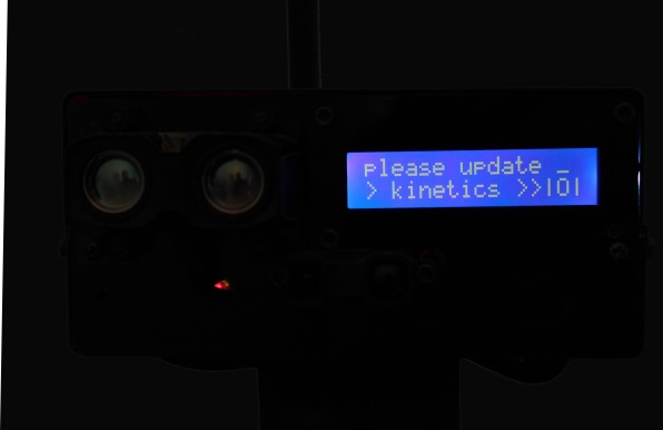
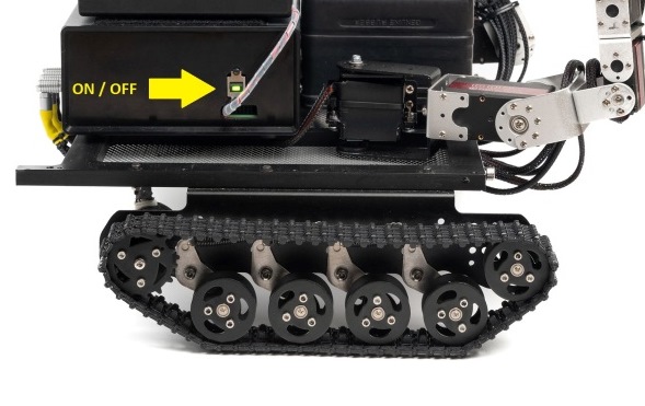
Fig.6. Powering-up KenjiX1.
As soon as it’s powered you will hear a booting sound, and you will be asked to “update kinetic parameters” on the LCD display (Fig.6.a). You should then on your laptop open the terminal program and start a SSH session with the provided IP-address (Fig. 7.a).
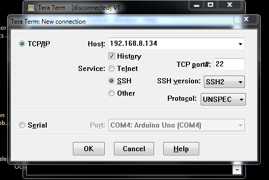
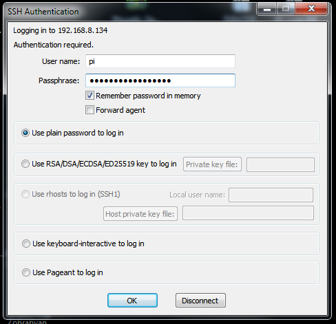
Fig.7. Remote connection to KenjiX1 via SSH.
Type in the “name” and “password” (Fig.7.b) and afterwards a successful connection with the KenjiX1’s onboard SBC aka (Raspberry-Pi) will be established (Fig.8.b). Entering the username and password, will boot to Linux console (Fig.8.). From now on, you can do pretty much anything via onboard SBC of Kenji X1.
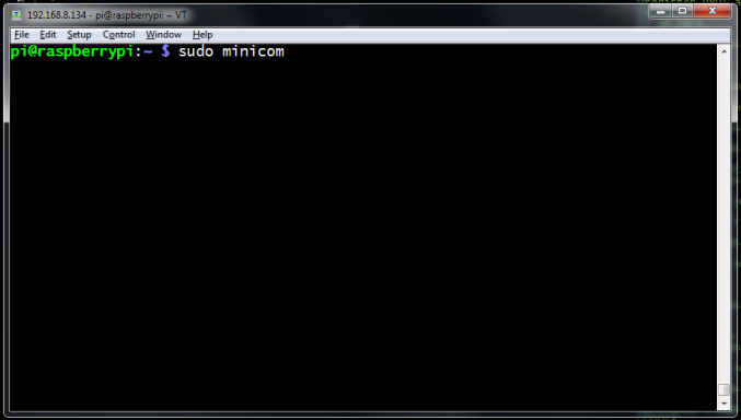
Fig.8. Remote Console on KenjiX1’s SBC .
We should establish one last communication node on KenjiX1 to make interacting with the robot platform fully functional. In console (Fig.8.) type-in the command “sudo minicom” and hit enter. You might hear several high pitch sounds coming out from the KenjiX1 and text appearing inside the shell. Congratulations (^_^) … now you gained access to roboDrive Engine. From this point and onwards there will be active connection to all network nodes, unless you as a user decide to break them.
Let’s make ourselves familiar with some of the roboDrive Engine’s instructions set. To view the “help/readme” info in (Fig.9.) type-in capital letter “H”. In “Run Control” we can configure the platform kinetic parameters: ground speed, tower rotation speed and so on.
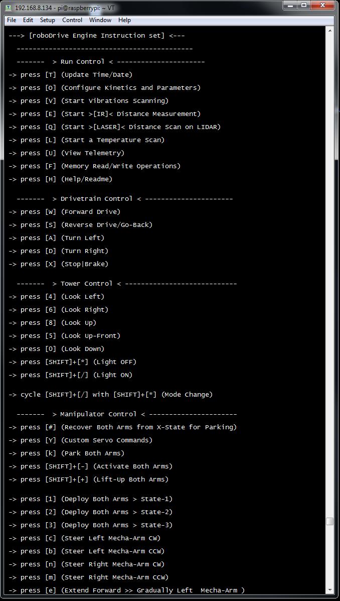
Fig.9. Updating kinetic parameters remotely.
Let’s type-in capital letter “O” to enter the menu. The first thing you’re being asked to “enter the vehicle ground speed”,” enter tower rotation angular velocity” and so on (Fig.10.) below.
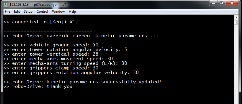
Fig.10. Updating kinetic parameters remotely.
Let’s enter all the needed kinetic parameters to the system as shown in (Fig.10): they take values in range (0 - 255).
- Enter vehicle ground speed = 50
- Enter tower rotation angular velocity = 5
- Enter tower vertical speed = 25
- Enter mecha-arms movement speed = 30
- Enter mecha-arms turning speed(L/R) = 30
- Enter grippers clamp speed = 20
- Enter grippers rotation angular velocity = 10
- Done!
Okay, let’s start driving forward with a minimal speed (50) and make ourselves familiar with control:
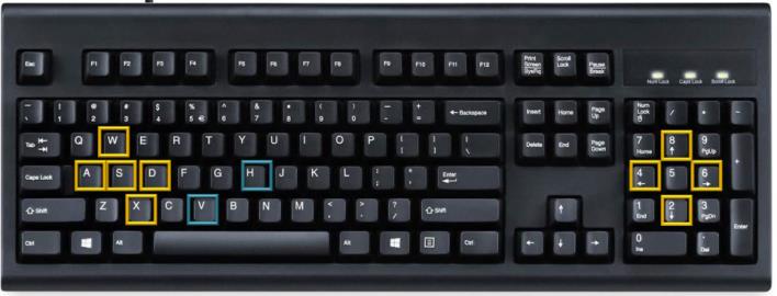
Fig.11. Control over the keyboard.
As illustrated in (Fig.11.), with the keys on the left (W, A, S, D, X) you can control the robot. It’s similar to PC-Gaming style, where you use your left hand to move around, and right hand for the mouse, which does the viewing around. Here is almost the same, you apply the left keys for moving around, and right keys, on the NumPad to look around up/down and and so on.
Measuring DC-Motor’s vibrations profile
Let’s start with measuring the vibration profile of the running DC-motor. I have prepared a test setup (Fig.12.), where the motor is powered over the Voltcraft laboratory power supply at about 10 Volts.
Fig.12. Faulhaber brushed DC-motor powered over the black lab. Power-supply at 10V.
As for now, the motor is running constantly and the shaft is spinning. Let’s consider that as an engineer we’ve got a technical task to measure the vibration profile of the brushed DC-motor remotely. In order to accomplish that task: we shall connect to robot, then we need to get robot driving close to the study object, engage onboard manipulator with the flat-surface conductive-probe and position it on the DC-motor’s frame, this is somehow similar to when pilots in space shuttle used to apply the manipulator to catch lost or malfunctioning satellites back then, and the last step get the data and evaluate it. This seems to be a lot … but we will manage it together (°_*).
Let’s start by driving KenjiX1 through my computer close to the area, where the test setup is located. In my case it is located at about 10 meters away, in facility so it will not going to take long. But it could be also that you control KenjiX1 somewhere on Solomon Islands. I am using the movement keys (Fig.11.) to drive and to navigate in space and approach the DC-motor slowly and stop somewhere at about 30-40 cm away from it (Fig. 13.).
Fig.13. Faulhaber geared DC-motor powered with the lab. power-supply unit (black) at 10V.
It’s time to deploy the conductive-probe and connect to the DC-motor’s metallic frame. Therefore, I am sending command “V” from my remote PC to un-park Mecha-arms. It takes second or two, and now both mecha-arms are in un-parked position (state-2), which would fit the best for this task. Normally there are several states (1-4) available to the user on KenjiX1, of course you can also code new ones as well.
Only un-parking and engaging manipulators don’t make a suitable contact with the DC-motor’s frame. I will switch from driving to manipulator steering control and try to steer around left/right up/down to make it work (Fig.14.). After several attempts, I managed to touch the frame of the DC-motor with the flat surface of the conductive-probes disc.
Fig.14. Positioning un-parked mecha-arms in state-2.
At this moment I have managed to get a contact with the DC-motor. Now, I just apply minor corrections and fine-tune the probe position by slightly moving left to right. The mecha-arm is pushing already the conductive-probe against the DC-motor’s frame, so there is a proper connection made.
Fig.15. Steering and minor adjustments of the mecha-arm and the conductive probe.
So far the surface to surface contact has been successfully established. Now It’s time to request data from the conductive-probe and save it inside our onboard SBC’s memory card.
There are two options here: you can either run the SBC with graphical user interface (Fig. 16.a) via “VNC Viewer” software or in console over “TeraTerm” software (Fig. 16.b), which I prefer more, but it’s just a matter of personal preference and you can do the same in both ways.
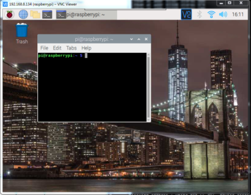
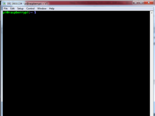
Fig.16. SBC graphical user interface (VNC viewer) left, and console access right.
By typing-in “sudo minicom –C userdata_file” command in shell, I ask system to run a session via minicom and to log all the data in a “userdata_file.txt” file. Here we just told the system to save our data points (which will be coming soon) to the generic text file called “userdata_file.txt”. Minicom splash screen on (Fig.17.b).
Fig.17. Connecting to roboDrive Engine console via minicom (a) in capture mode.
The housekeeping stuff is done by now, and we can request 10K data-points from conductive-probe which currently is measuring the vibrations generated by the running DC-motor.
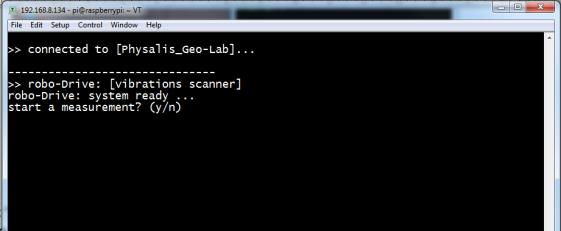
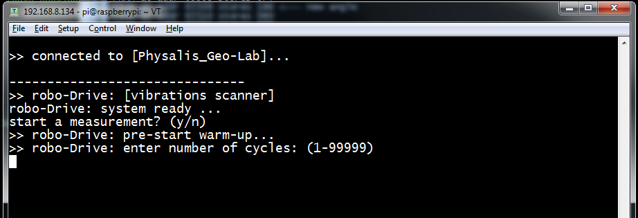
Fig.18. Requesting 10k data-points to be streamed to us and saved onboard.
Start data stream by typing-in “V” to run “scanner setup” (Fig. 17.a). It will appear in shell (Fig.18.b) type “y” for confirmation, and then the desired amount of cycles: “10000” and hit “enter”. As soon as you hit enter, you will see the data stream burst directly inside the shell. That is the real-time data being dispatched to us and also saved onboard. Three types of data points are being registered over the time. The actual amplitude, lowest amplitude (threshold) and highest amplitude (threshold). We measure in time domain, and thus we see a “time [ms]” value on far right column. Nice!....
Fig.19. Data streaming from conductive-probe over time.
As mentioned above the conductive-probe is sending the requested amount of measurement cycles to us. As for now, we can relax and have a cup of coffee. Depending how many measurement cycles you request the time can be longer or shorter, so after minute has passed, and the streaming is over with a message “Scan Complete”.
But all this raw numbers and cryptic look is not exactly what we were hoping for. I guess it will be much better to have something which we can view graphically, and maybe share with others or e bed in report.
Okay, if you remember, before starting the data streaming we asked the system to capture and log our interaction with KenjiX1 and save it in our file named “userdata_file.txt” which is now sitting inside the KenjiX1’s onboard SBC’s memory card.
Setting-Up Data-Dispatch
Let’s get that data-file transferred to our PC where currently me, or you “KenjiX1’s operator” residing now. On my PC, I can achieve that by typing inside windows PowerShell
“pscp [email protected]: home/pi/userdata_file userdata_file.txt” command
Please note you should enter the provided password for the KenjiX1’s onboard SBC. The file will be copied to the “D:\Users\Arhitect” folder in my example, and on your PC, depending where your path is. In PowerShell, check it via “pwd” command where your path is. Please install “putty” software for using “pscp” aka “putty secure copy” command and much more in PowerShell. https://documentation.help/PuTTY/pscp-usage.html
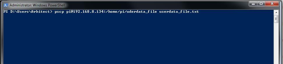
Fig.20. Getting measurement data shipped to us via PowerShell over the network.
The file has been copied remotely to my PC and is located in directory “D:\Users\Arhitect”. Because we changed the working environment from Linux to Windows, if you open this text file, it will look “fuzzy” (^_^) (Fig.21.a.).
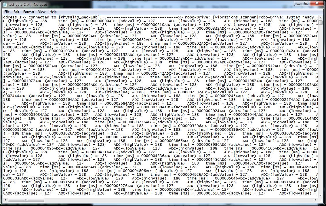
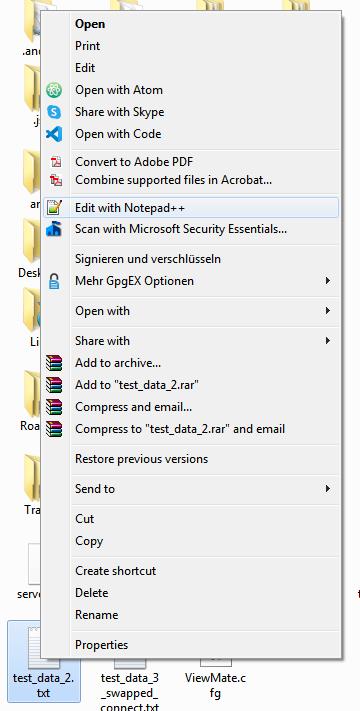
Fig.21. Using Notepad++ to change the EOL termination.
We should make an “EOL” correction for Windows machines. In context-menu, click on “edit with Notepad++”, if you don’t have Notepad++, just get it from here https://notepad-plus-plus.org/downloads/.
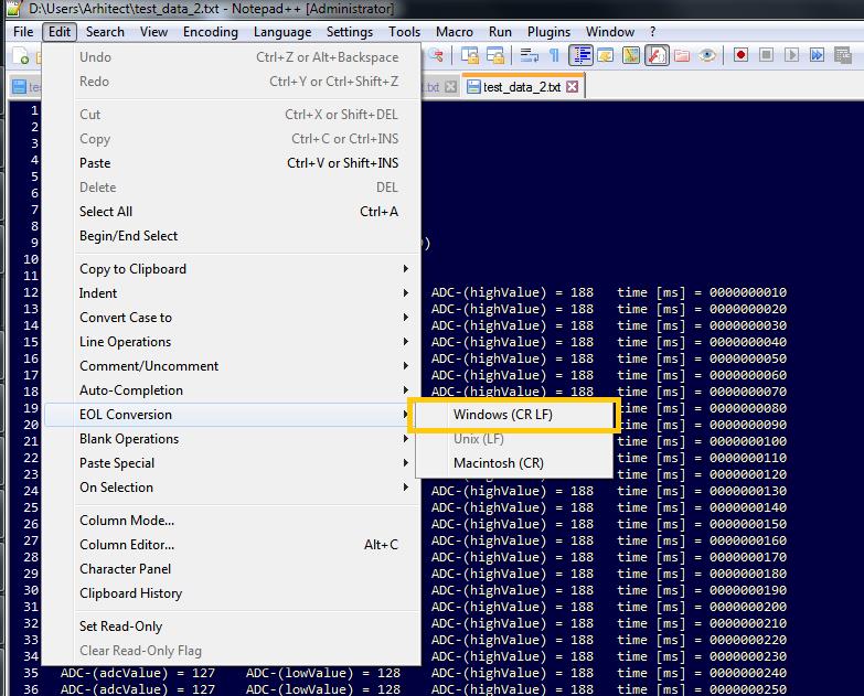
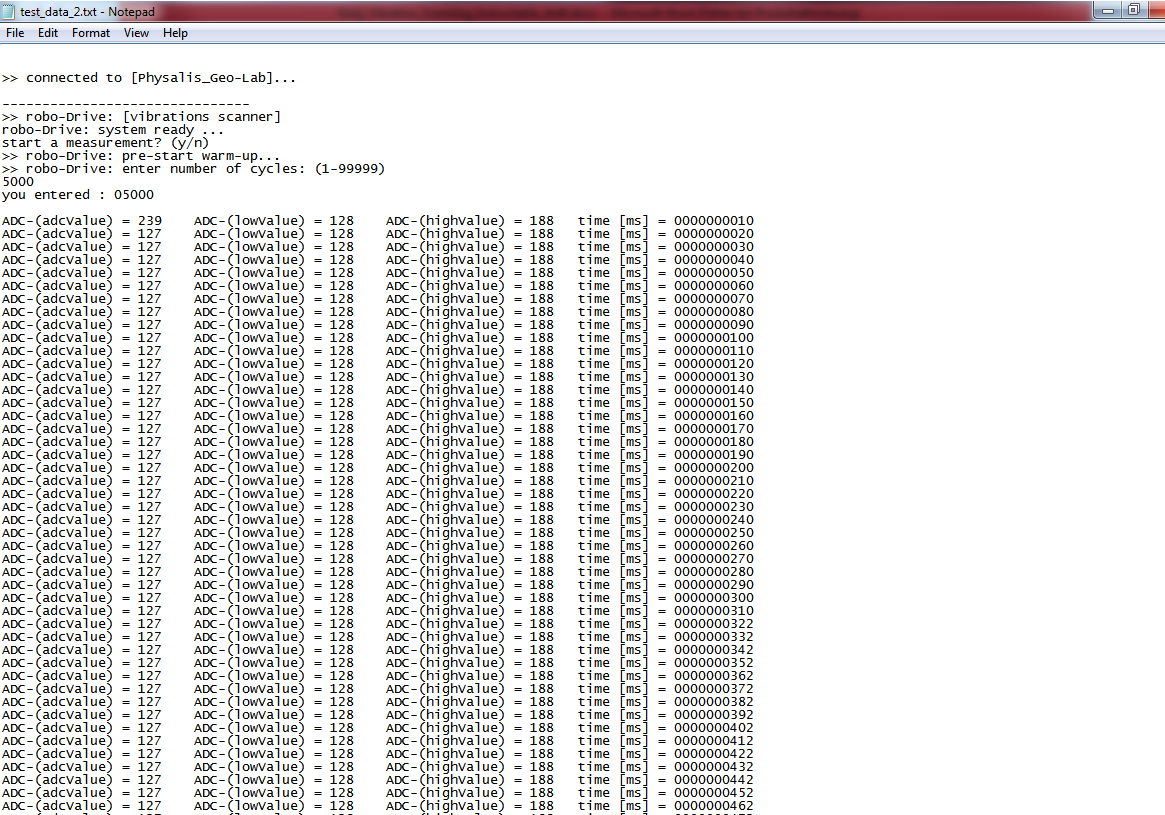
Fig.22. Changing the EOL conversion to Windows(CR LF).
Click to edit the file in Notepad++ and when its opened up, inside the program, go to “menu” then “edit” then “EOL Conversion” and hit “Windows(CR LF)” and save the file via “CTRL-S” and close the Notepad++. That way, we changed the “end of line” termination to the windows style. If we open the file now, it will look similar to (Fig.19.) data stream.
Visualizing Measurement Data
There is handful of ways to visualize measurement data, and they all are good in their own way of doing it. At the end of the day it’s up to you how you are visualizing your data. I have chosen OriginLab Pro. It is really great software which has been around since ages. Especially if you’ve worked with scientists, you might already come across, because it’s really popular in those circles.
We will start by running the software on PC and normally it will open up a new and empty book as

Fig.23. Running OriginLab Pro software on PC.
I will import the “userdata_file.txt” which we copied to my PC. OriginLab has an import wizard under the section “menu” then “File”. At first click once on an empty data-book and make it active, then go to import and import the file as “single ASCII” or you can also try “import wizard” if you have issues importing data through “single ASCII”.
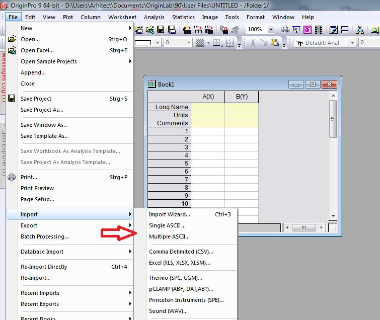
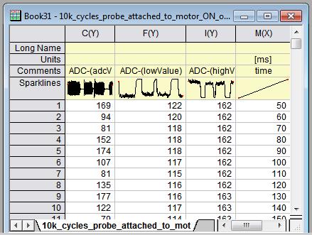
Fig.24. Running OriginLab Pro software on PC.
The “import wizard” gives you more options to manipulate and you can change things like the “delimiter” names, and more. You can try various scenarios to find the best options which will satisfy you the most. Eventually after successful import you can nearly see some tiny thumbnails at the top of each column we imported.
Each column has its dedicated name in OriginLab software, so as seen the columns C(Y), F(Y), I(Y), M(X) are the 3 x amplitudes from our conductive-probe, and as you remember we are working in time domain and therefore the last one is the time. You should explicitly tell the program which axes should be plotted as X-Axes and which ones as Y-Axes. I will tell the program to plot the dependency
𝑓([𝐶(𝑌) 𝐹(𝑌) 𝐼(𝑌)], 𝑀(𝑥))
Which means that “M(X)”dataset, which has all the time values inside will be plotted as X-Axes and all others “C(Y), F(Y), I(Y)” which are holding the vibration waves amplitudes as Y-Axes. For better overview I will divide down the M(X) dataset by 1000 to get time in seconds. Otherwise the values of the X-Axes are too high.
In total we will plot 4 datasets in one graph:
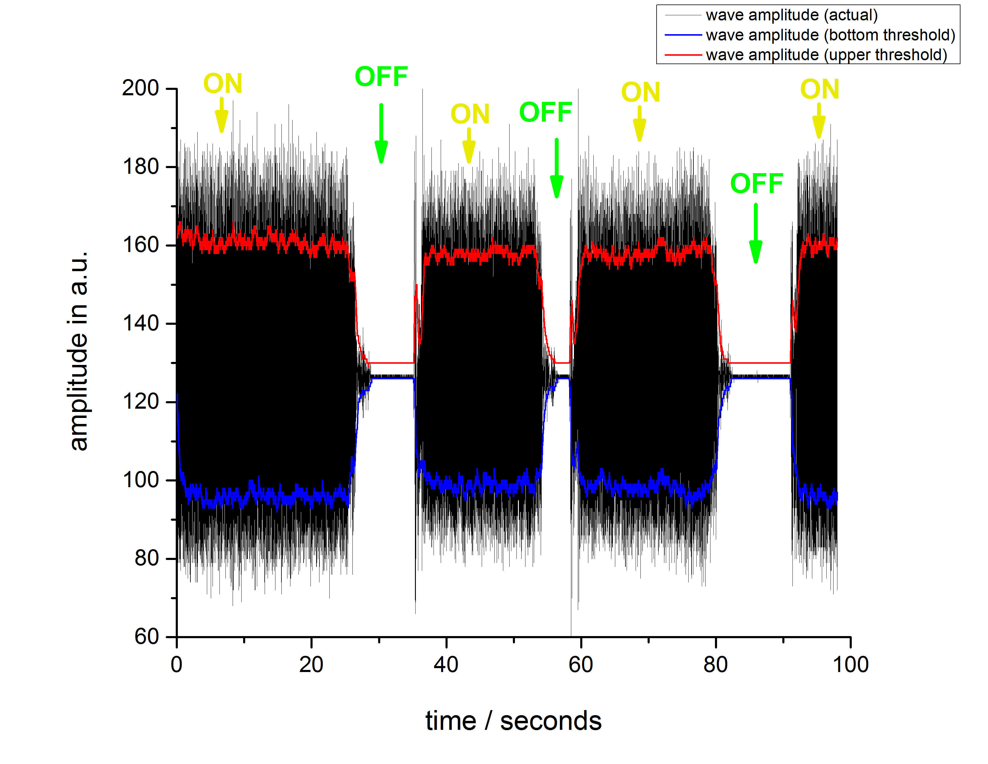
Fig.25. Running Brushed DC-motor vibration profile measured on Kenji X1 robot.
Finally, we have it … in (Fig. 25.) we visualized the measurement data and created a beautiful and informative graph from it, which you can include in your semester work, or classwork. But along the way, you also learned a lot more, and now you can navigate yourself with confidence in such complex interconnected systems and in between communicating nodes.
But wait! … (°_°)…
This is not yet the end, this is just the beginning, and now with all this knowledge in your pocket you can apply the stuff you learned here to study other interesting things, excitation sources, get creative. Spending quite some of my time to create this instructable after a regular job, so there might be places where something is written goofy, or something I forgot to mention.
I hope that you liked this instructable and could learn something new from it.